Orshansky Article:
Who Was Molly Orshansky and How Did She affect Assessing?
by JOSEPH M. TURNER, CEO,
Michigan Property Consultants
Published in The Michigan Assessor, July 2008
The Person
The professional work of Mollie Orshansky has tremendously affected our American government - and through federal determinations and decisions - property tax burdens in the state of Michigan. My guess is most assessors working in this state have had their property values adjusted based upon the influence of Mollie Orshansky and that most assessors have never heard of her.
So who was Mollie Orshansky? According to federal documents, Mollie Orshansky was a graduate of Hunter College with a degree in mathematics and statistics who worked for both the U.S. Department of Agriculture and the Social Security Administration. Social Security Online, an internet gate for the Social Security Administration states she developed the official measure of poverty used by the U.S. government www.ssa.gov/history/orshansky.html (May 27, 2008).
Guidelines Ms. Orshansky developed have withstood the test of time. They are the basis for the poverty criteria used in determining eligibility of applicants for Michigan’s “Hardship Exemption” pursuant to M.C.L. 211.7n. Ms. Orshansky’s work also is believed to have influenced legislation related to President Lyndon B. Johnson’s War on Poverty in the 1960s.
Basis for defining the poverty level
The basis for the modern definition of a households living in poverty begins in 1955, with a U.S. Department of Agriculture study on minimum diet, food consumption and the cost of food. A basic idea behind work at the Department of Agriculture was to identify several food consumption patterns and classify them based upon dietary needs and costs. One of the identified diets was called the “thrifty food plan.” This plan for food consumption was “designed for temporary or emergency use when funds are low.” (See www.ocpp.org/poverty/how.html for more details). The “thrifty food plan” was a minimum diet one could subsist on, but judged insufficient for long term dietary needs. As part of its research, the Department of Agriculture determined in its 1955 study, that a family of three or more persons spent about one third of its available income on food.
Following her tenure with the Department of Agriculture, Ms. Orshansky took a position with the U.S. Social Security Administration. There she was assigned the task of creating an official definition for poverty. She established poverty thresholds in 1963-1964 and published an analysis in a January 1965 Social Security Bulletin article. The definition was stark, according to Professor Timothy Taylor of Macalester College. In his lectures contained in “Economics, 3rd Edition,” poverty as defined, meant that only enough money existed for basic necessities. If one were to spend excess money on items in one category of basic needs, then there would be insufficient funds to purchase items in another.
To establish poverty thresholds, Ms. Orshansky used the “one-third / two-third” proportionality identified in the Department of Agriculture food studies. “In effect, she took a hypothetical average family spending one third of its income on food, and assumed that it had to cut back expenditures sharply.” ... “When the food expenditures of the hypothetical family reached the cost of the economy food plan,” (thrifty plan) “she assumed that the family spending on non-food items would also be minimal but adequate.” ... “She derived poverty thresholds for two-person families by multiplying the dollar cost of the food plan for that family size by a somewhat higher multiplier (3.7) also derived from the 1955 survey. She derived poverty thresholds for one-person units directly from the thresholds for two-person units, without a multiplier. The base for the original thresholds was calendar year 1963.” (http://aspe.hhs.gov/poverty/papers/HPTGSSIV.htm May 27, 2008)
Changes since 1963
Since her original work, poverty calculations have been expanded from seven person families to nine person families. In addition, the matrix needed for the detailed scientific work contained 124 poverty thresholds. In 1981, the number of matrix thresholds was reduced to 48. The differential which existed between farm and non-farm families was eliminated “by applying non-farm poverty thresholds to all families. (I.D. page 2 of 3). At the same time there existed a distinction between poverty in male headed households and female headed households. That was eliminated by averaging between the two.
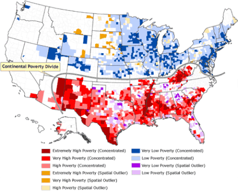
Here is a snapshot of the geographic distribution of income according to a study in 2007. The graphic was created by using federal poverty statistics for 2000, articulated at the county level.
We intuitively recognize there are market forces at work which affect poverty. Professor Taylor, addressed “inequality” of household income and the way money is distributed. In one lecture, he described a recent trend in households which tends to focus money within some households and diminish what had been an equalization trend in the past. It works this way. Historically, a high income earner such as a doctor, lawyer or business professional, might very well marry a low income earner. An example would be a doctor marrying an employee. The union of a high income and lower income person would tend to mitigate inequalities, since the combined household would eliminate a lower income household.
However, recently, there has been a trend for high wage earners to marry other high wage earners. For example, a doctor might marry another doctor. In such a case, inequity in terms of annual income between households is increased, not decreased.
By the way, the face of poverty has changed considerably since Orshansky developed the working definition for poverty. When the first snapshots were taken using Orshansky’s criteria, the poor were the elderly in our society. Today, the poor are often children living in single parent households. Below are graphics illustrating high and low income areas of the U.S.Areas with low poverty - at least one standard deviation below the national average
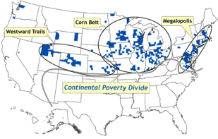
The snapshot of wealth or higher income households was developed using statistics from calendar year 2000 at the county level. What do you think the picture would look like today,after only eight years and many plant closings ?
Areas in U.S. with exceptional poverty levels
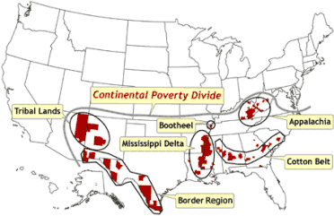
Using county level statistics, this map highlights areas in the U.S. with 2000 poverty levels at least two standard deviations higher than the national average.
Source for both images: The Topography of Poverty in the United States: A Spatial Analysis Using County-Level Data From the Community Health Status Indicators Project, James B. Holt, PhD, MPA, Preventing Chronic Disease, Volume 4: No. 4, October 2007 http://www.cdc.gov/pcd/issues/2007/oct/07_0091.htm